We system integrators must test our control system configurations. Ideally we thoroughly test them before systems are delivered. Simulating inputs based on outputs is a key tool to perform these tests.

Traditionally, the FAT (factory acceptance test) has focused on a thorough test of the hardware along with the controller and HMI configurations to run on that hardware. With the advancement in emulation software, it now often makes sense to split the FAT into separate hardware and software tests, with the software test utilizing simulation logic.

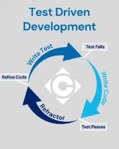
There is a coding concept called Test Driven Development. The idea is each code module should be designed to be independently testable – to be easily demonstrated to have met all its requirements in isolation. Then moving up from there, groups of modules can be tested together, etc… For formal TDD, the following order should be followed for each module:

• Define its requirements.
• Create the module definition (including defining inputs and outputs) but with no internal code.
• Develop a test routine to call that module with various inputs and verify its results match requirements.
• Run the test routine on the empty module, and verify the test fails. (this is an initial test of the test).
• Code the module.
• Run the test routine on the module again and make sure it passes.
• Many compilers retain the test modules as a permanent part of the code, and run all of them when the application is re-compiled to verify no code has been inadvertently broken.

In programming control systems, it is not practical to exactly follow the formal TDD model, but we can learn from those concepts. Specifically:

• The primary goal of simulation is to verify that configurations meet requirements. Therefore detailed “target for success” specification documents must be written, and approved by the customer and sometimes third party equipment vendors or engineers. These documents often include system requirement specifications, detailed design specifications, control narratives, Cause & Effect Matrices, Piping & Instrumentation Diagrams for HMI testing etc. They should be written to include granular requirements that can be easily tested with clear pass/fail results.
• Large chunks of code which have too many permutations to practically test should be separated into smaller modules which each have few enough permutations to reasonably test.
• Simulation logic should be coded and performed from the beginning of the configuration process. Use it to test the configuration all along its development. This is especially important for components that will be copied to many instances. To reduce repetitive work later on, one iteration of each type of control module should be extensively tested before copying it. That should include everything about the CM – interlocks, tuning, alarms, main HMI display objects, popup faceplates, etc…
• Include simulation code in the final PLC program delivered to the customer, with a soft switch to disable it when using real inputs. If the system is later expanded or extensively modified, that simulation code can then be re-used. It can also become part of operator and/or technician training systems, should the customer be willing to pay for such a system.

Input simulation logic should only look at outputs or other inputs – not internal information such as setpoints, modes, etc. An exception to this guideline is simulation jump request logic (see below).

The simulation must allow normal working logic to be tested, but also support exceptions testing – especially exceptions which are specified to result in an action such as tripping an interlock. These include device trips (motor fails to run or valve fails to open), bad signal qualities, module & communication faults, PV deviations from acceptable ranges, etc… My usual approach is to have the simulator run everything as expected by default, and manually initiate exception conditions. I then have a global simulation reset request that puts all the fault conditions back to their normal good states.

For Rockwell systems programmed in Studio5000, I typically employ simple IO handler AOIs (add on instructions) for each type of data. They all attach to a common global UDT (user defined type) that includes simulation mode, a simulation reset pulse, etc… When in simulation mode, all inputs ignore their physical input attachment and instead look at their simulation inputs. Outputs do not need to simulate – however they should disable their physical outputs when in simulation mode. This prevents inadvertent unsafe operation of real equipment based on simulated inputs.

Some PLCs allow writing to input data when those inputs are not connected. However if you use that method, simulation will not work when real inputs are connected. Therefore I prefer to switch between simulated and real input values in those IO handler AOIs.

DI Simulation

For Discrete Inputs my IO handler includes simulation on and off delays. I attach the expected state to a simulation input on the IO_DI block, and those delays dictate how long from when that input changes state until the IO_DI result changes to match it. Those delays can be manually increased to simulate faults.

Many DIs are expected to change state based on process conditions (a valve closed limit switch should simulate on when the valve output is in the close command state). Others should always be on, and an off state is always an exception (like emergency stop pushbuttons). The simulation system should allow both kinds to normally simulate expected conditions but allow exceptions for testing.

I also often add a simulation exception test integer to the DI AOI. When set to a non-zero value, it counts back to zero by one each scan. If negative, it overrides the regular simulated input with the off state. If positive, it overrides the regular simulated input with the on state. At zero it goes back to normal. This can be added to the DI popup faceplate with an animation so it is only visible when simulating.

AI Simulation

Analog Input simulation has a vast array of possibilities. I typically include non-linear responses, ramping, and noise in my simulations, but not hysteresis.

There are generally two types of AIs to simulate:

• AIs expected to act as a mathematical function – to return a value based on an output where the previous simulated input is not a factor (other than ramping). An FT (flow transmitter) with an associated FCV (flow control valve) or variable speed pump is the archetypical example of this. For FCVs I like to run the valve output through an X^Y function with the exponent around 0.9 to simulate slight non-linearity (more FT response from 10-15% than from 90-95%), and an adjustable multiplier. I also include a switch to simulate zero flow when the output is very low (like < 5%) or a device such as a pump is not running. That is sufficient to thoroughly test a flow PID loop. So for a 0-100% FCV as simulation input to a 0-200 GPM FT, I would set a pre-exponent bias of -5%, and a multiplier to around 3.32 because (100-5)^0.9×3.32=200.

I typically simulate motor current AIs with logic in my motor & VSD (variable speed drive) IO blocks to perform current simulation somewhat realistically with inrush currents, steady-state currents, slightly increased current when accelerating, etc.

• Other AIs strongly depend on their previous values – these include levels and temperatures. In those cases a simple feedback from the output through a function to the input is insufficient. Instead, process conditions that add to the level should simulate addition, and processes that remove from the level should simulate with subtraction. If the system includes flow AIs in or out, the result of those simulations can be used to simplify level simulation logic.
• Temperatures: Have a slow exponential decay filter to always move the temperature toward an ambient value each scan. To simulate heating, a realistic model is to add a small fraction of the heat output to the simulated temperature each scan. Depending on the type of cooling, you can subtract a small fraction of the cooling output each scan, or (for cooling towers or other heat exchangers that cool to near ambient conditions) shorten the time constant of the ambient filter based on the speed of the fan. I ignore the additional cooling from vaporization unless doing a fully realistic model – but in that case it would decay toward the simulated ambient dew point instead of ambient temperature.

In all cases, it’s helpful to clamp the simulated input to the analog input block’s process scale (for PlantPAx 5’s PAI – “process analog input” – that would be Cfg_PVEUMin and Max). When feeding typical AI blocks that include scaling from a raw range such as a PAI, the input handler should de-scale its simulated PV back to raw units. For example if a PAI scales 4-20mA to 0-200 GPM, and the simulated flow is 50 GPM, the block should de-scale that to 8mA and pass that value to the PAI’s raw input.

If simulated hysteresis is desired, the IO_AI handler should have a hysteresis amount setting. Then the simulated value should only ramp toward the simulation input if that input is greater than the hysteresis setting away from the simulated value. For an FCV→FT simulation with 2% hysteresis, when raising the FCV to 20%, the FT would settle at the 18%FCV flow, and when closing the FCV from >22% down to 20%, the FT would settle at 22%FCV flow. A physical analogy of that behavior is a control valve moved by an actuator in a loose slot instead of a well-fit hole.

Random numbers for noise – I use the LCG (“linear congruential generator”) for a pseudo-random number to add noise. The LCG produces a pseudo-random integer from 0 to 2³¹-1. The initial value “n” should be seeded on first scan, which I do from the processor’s clock microseconds. Then every time an AI executes, it applies this math to n: n(new) = ((n × 1103515245) + 12345) modulo 2³¹ (16#8000_0000 or 2147483648). It then multiplies that by 0.0000000009313225746 and subtracts one to yield a pseudo-random REAL between -1 to +1. All the AIs add a small multiple of that to their raw values to realistically simulate random noise.

Jumping the Simulation

For processes where transitions to be tested occur minutes or hours after an event, simulation jumps are desirable. This is particularly important for batch processes. This allows users to test batch logic in a few minutes when the real-world batch might take multiple hours or days. I put a single “jump sim” button on the batch popup that is only visible when simulating and the module is in a state where jumping is meaningful. For states waiting on a time to elapse, I have the jump logic set the accumulator to 5 seconds less than the target time (preset). For states waiting on totalizers, I execute the simulation logic after the periodic flow totalizer but before the batch logic accumulates its scan-total. I then override the scan total so that the new batch accumulated total is 5-seconds’ worth of flow less than the target.

This allows test users to jump without knowing anything about the programming, such as where timers or batch total accumulators are in the code.

Realistic Modeling

The above methods are sufficient to thoroughly test configurations against typical specifications, including ensuring PID loops are pointed in the correct direction.

If more realistic simulation is needed, this can be done, but represents a huge increase in time & effort. Large amounts of data about the process and instrumentation must be collected, coded, and populated in arrays in the controller. These include valve and pump curves, pressure drops across significant pipe lengths, thermal mass of any fluids and containers involved in temperature control, etc.

In general these realistic models depend on iterative calculations to produce realistic results – a simple example would be a constant speed pump and FCV controlling a flow to simulate both flow and pressure, where the flow and pressure affect each other. In this case even if pressure is not a point in the system, it must be simulated for the model to work. The simulation code should calculate pump discharge pressure before the FCV from the pump curve based on flow (pulling values from FGEN or similar array interpolation). Then it simulates flow from that discharge pressure based on the valve’s position and valve curve FGEN. After a drastic change it may take a few scans to settle out, but with proper ramping/filtering, a realistic flow -vs- pressure -vs- FCV position relationship can be accurately modeled.

Partner With Our Process Solutions Group

The process control and simulation techniques outlined in this guide represent just a fraction of our team’s technical capabilities. At Cross Company, our Process Solutions Group engineers apply this deep industry expertise directly to your unique challenges. Whether you are validating new logic or modeling complex systems, partnering with our experts ensures you have the right strategies in place to improve product quality, raise operational efficiency, and significantly lower risk. Contact us today to see how our engineering team can optimize your next project.