How to tune a PID loop
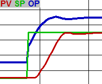
The art of tuning a PID loop is to have it adjust its output (OP) to move the process variable (PV) as quickly as possible to the set point (responsive), minimize overshoot, and then hold the variable steady at the set point without excessive OP changes (stable).
Definitions
- PID = Proportional, Integral, Derivative algorithm. This is not a P&ID, which is a Piping (or Process) and Instrumentation Diagram.
- PV = Process Variable – a quantity used as a feedback, typically measured by an instrument. Also sometimes called “MV” – Measured Value.
- SP = SetPoint – the desired value for the PV.
- OP = OutPut – a signal to a device that can change the PV – frequently a valve, damper, or a pump speed reference. Often called “CV” – Controlled Value.
- Overshoot = when the PV moves further past the SP than desired.
- A PID loop in manual (as opposed to automatic) only changes its OP upon operator request.
- A loop in remote (aka cascade) has its SP automatically adjusted by external logic. In local the SP is only changed by the operator.
- A direct acting PID loop increases its OP in response to increasing PV, while a reverse acting loop decreases its OP. “Normal” loops are reverse acting. Loops controlling level or pressure via a valve on an output, or temperature via cooling are generally direct acting – “backwards” loops.
- Error = the difference between PV and SP.
Already know the basics of how to tune a PID loop? Check out our article Advanced PID Loop Tuning Methods
See How Our Team Can Help Improve Quality, Increase Efficiency, And Reduce Risk
Three Basic Tuning Parameters of a PID loop
Note: for demonstration purposes the charts below show the individual responses of the actions where the PV is NOT affected by the OP. Normally the PV would be affected by the change in OP & would therefore be brought back toward the SP as a result of the OP’s response.
Gain
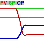
Also called proportional band or P-gain, the gain determines how much change the OP will make due to a change in error (from a PV change and / or an SP change). This mainly corrects the OP based on upsets as they happen. “Gain” implies that a larger number will have more effect. “Proportional band” implies the opposite. P-Gain = 100% / P-band.
Reset
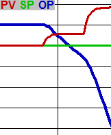
Also called integral or I-gain, the reset determines how much to change the OP over time due to the error (regardless of the direction of movement of the error). This brings a stable PV that is off SP toward the SP. Reset or I-gain implies that a larger number will have more effect. Integral implies the opposite. Reset [resets per minute] = 60 / Integral [seconds per reset].
Preact
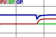
Also called derivative or D-gain, the preact determines how much to change the OP due from a change in direction of the error or PV. Acting on the PV, rather than the error, is an option in some loops That is generally better because it is undesirable to bump the OP when the SP is changed. It is called preact because it allows the loop to “anticipate” upsets as they begin to happen and react quickly.
Actions working together
When the PV is approaching the SP, Proportional and Integral work in opposite directions to cause the PV of a properly tuned loop to get to the SP quickly without excessively overshooting. For a typical reverse-acting loop, the proportional will try to close the OP as the PV rises toward the SP, but the integral will try to open the OP because PV is below SP. As the PV gets closer to the SP, integral action decreases resulting in the PV smoothly decelerating into the SP.
Initial Loop Tuning
The goal of tuning a PID loop is to make it stable, responsive and to minimize overshooting. These goals – especially the last two – conflict with each other. You must find a compromise between the goals which acceptably satisfies them all. Process requirements and physical limitations will determine the balance between the amount of acceptable overshoot as well as the demand for responsiveness. The primary factors which dictate the limits to responsiveness of a loop are:
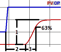
- The amount of PV change resulting from an OP step change.
- The time from when the OP changes until the change starts to be seen in the PV,
- The time for the PV to reach its new level. Because the PV usually approaches its new level asymptotically, for that time constant we frequently use the time it takes the system’s step response to reach 1-1/e, or about 63% of the distance from the initial to its final value.
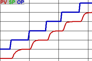
Before tuning a loop, make sure you have a good trending package. Watch the PV, SP, OP and other outside variables you suspect might influence the PV together. Characterize the loop by making step changes in manual through the range of the OP and back, and make a note of these three factors. Stepping through the range in both directions is valuable to quantify the linearity and hysteresis of the system.
Linearity: If the same change in OP through the whole scale results in a similar change in PV at each point, the system is linear. But if a change on one part of the OP range results in more PV change than the same OP change in a different range, the system is non-linear.
Hysteresis: Some devices will yield a different PV for the same OP depending on whether the OP went up or down to get there. A valve might allow 25 GPM through after moving from 20% to 30%, but 30 GPM after moving from 40% to 30%.
Two Basic PV Categories: Particle and Bulk
Particle properties are those where a fluid in a pipe may have different properties in different areas, so that the fluid must be mixed or moved to change the property at the PV measurement point. Particle properties include temperature, pH, conductivity, etc. These tend to have a significant delay between a change in OP and the beginning of the change in PV (#2 above), and therefore might benefit from derivative action.
Bulk properties describe the state of the fluid as a whole so that it all changes everywhere in a pipe or vessel (for practical purposes) simultaneously. Examples: flow, level, and pressure. Generally these PVs begin to show the result of an OP change immediately (even if the time constant to complete the change is long) and do not need any derivative.
Another categorization of PVs: some (such as flow) increase when the OP increases and decrease when the OP decreases. These should be characterized as shown above – they typically need more integral and minimal P-gain. For others (such as level) the direction (slope rather than value) of the PV is relative to the OP. For the latter, a characterization is more subtle – you want to characterize the slope of the PV for various OPs instead of its value. These sometimes need moderate-to-high gain and less integral.
Starting Parameters
Loops where the PV changes quickly due to a change in OP (flow, or pressure or level in vessels with fast turnover) should have low P-gain (perhaps 0.2) and higher reset (1.5 – 10 rpm). Loops where the PV changes slowly, or changes its direction of movement due to change in OP (temperature and level in vessels with slow turnover) typically need high gain (3 – 100) and low reset (0.05 – 0.3).
These recommended starting parameters are based on the input and output ranges being the same. Some controllers handle tuning parameters based on percent of span, while others do not make this correction. If the spans are different, corrections would have to be made to the parameters themselves. For example, if the flow through a pipe can be from 0 – 10,000 gpm, and you are adjusting the speed of a VFD from 0-100%, the starting gain and reset would need to be 0.004 and 0.02 instead of 0.4 and 2.0.
There are numeric methods where the natural resonant frequency of a system is determined and parameters set accordingly, but an iterative, intuitive approach may be more useful:
- Start with a low proportional and no integral or derivative.
- Double the proportional until it begins to oscillate, then halve it.
- Implement a small integral.
- Double the integral until it starts oscillating, then halve it.
That will get the constants close to where they need to be for fine adjustment. Don’t hesitate to put the loop back in manual if the loop goes crazy or while studying the trend.
Fine Tuning
To achieve the goal of a responsive and stable loop with minimal overshoot, the tuning must be tested in response to upsets and at steady state. Upsets can be induced by:
- Changing the SP
- Putting the loop in manual, changing the OP, then returning to automatic
- Externally causing a change to the PV
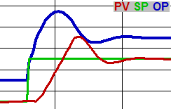
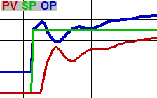
Once the PV has stabilized at its SP, upset it by stepping the SP. Even a very small change is useful here. The proportional will cause an immediate jump in OP, then the integral will cause the OP to continue ramping in the same direction. When the PV starts to move, the proportional will cause the OP to move back the other way, and the integral action will diminish as the PV approaches the SP. Overshoot is often caused by too much integral and/or not enough proportional.

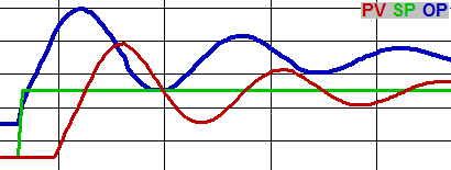
The OP needs to start moving back the other way well before the PV reaches the SP. The amount of time between the peak and the PV hitting the SP depends on the nature of the loop. If the peak comes too late, you need more proportional or less integral. If the peak comes too early, you need less proportional or more integral. An early peak will result in the PV leveling out before it reaches the SP, causing the OP and PV to swing on the way to their new steady-state values.
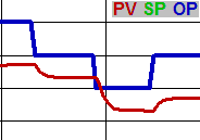
Once the loop is roughly tuned, put it in manual and change either the SP or OP, let it stabilize, then put it back in automatic. The loop will then move the PV to the SP, but with integral only – without the initial OP pulse from proportional. If the OP moves too slowly, you need more integral. A long delay between the change in OP and the end of the resulting change to PV dictates a lower integral value. Introduce derivative if you see that a bump in OP would be beneficial when the PV changes direction at the beginning of an upset.
This is an iterative method – every change in one parameter changes the ideal value for the other parameters. Go back and forth between upset methods and steady state stability, and make sure you check the tuning for the full range of possible SPs, If the system is non-linear (see above), a loop that is stable at higher flows may swing wildly at lower flows, and a loop that is responsive at low flows may be sluggish at higher flows. A PID loop with a control deadband can sometimes achieve acceptable control despite this challenge. See other ways to deal with valves and dampers with deadband in Advanced PID Loop Tuning Methods.
Diagnosing the Cause of Oscillations
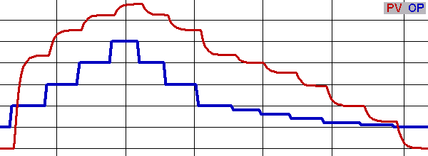
If the OP and PV peak at the same time, the oscillation is proportional-driven.
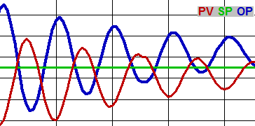
If the OP peaks when the PV is crossing its midpoint & visa versa (so that the PV and OP waves are 90° out of phase), the oscillation is integral-driven. Some oscillations are driven by other factors in the system – put the loop in manual to see if it continues to oscillate if you suspect the loop you are tuning is not causing the oscillation.
Sometimes oscillations are acceptable. For example, the goal of boiler drum level control is primarily to avoid tripping on either low or high level. A moderate amount of oscillation at steady state is a good trade-off to get enough additional responsiveness to avoid tripping following significant upsets.
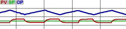
Note that actuators (especially motorized valves) with deadband and/or limited duty cycle will ALWAYS swing when attached to a traditional PID loop regardless of tuning parameters. You can tell this is happening by looking at the trend – the PV will be flat while the OP is ramping down (due to integral), then the PV jumps to the other side of the SP, and the pattern reverses. See how to deal with valves and dampers with deadband in Advanced PID Loop Tuning Methods.
Balancing the Tuning Goals
A properly tuned loop balances the demands of stability, responsiveness and low overshoot. Tune the loop by adjusting the three tuning parameters so that the loop responds well in a variety of upset and steady-state situations. Some Advanced PID Tuning Methods may be necessary if challenges such as non-linearity, deadband, hysteresis or measurable external upsetting events prevent the loop from being satisfactorily tuned with the basic methods described above.
Work With an Expert
If you are experiencing issues with tuning your PID loop we encourage you to reach out to one of our process solutions experts. While this guide is intended to help you tune your PID loop and troubleshoot common issues, this is not an exhaustive list. Please contact us today to discuss your application and specific issues you may be having with your PID loop.