Advanced Methods for Tuning a PID Loop
A PID loop adjusts its OP to maintain its PV at its SP. Some PID loops cannot be satisfactorily tuned by adjusting the three primary constants. When combined with good basic tuning, advanced methods can improve stability, responsiveness, and limit overshooting. See The Basics of Tuning PID Loops for suggestions on basic tuning and a list of common terms and definitions.
Cascade
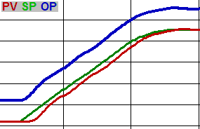
The basic PID cascade is a pair of PID loops where the OP of the master/primary loop sets the SP of the slave/secondary loop. For example, a tank level PID loop might have an OP in k#/H flow rather than % to a valve. That master OP is sent to the SP of a slave PID loop controlling flow. This is ideal when the master loop must be slow but the slave loop can be very responsive – the slave loop enables the OP of the master loop to be linear and have no hysteresis, even if the OP of the slave loop suffers from those deficiencies.
Ideally, the scale and units of the master OP should be the same as the PV and SP of the slave loop. That allows direct transfer and tracking without scaling. With older systems which require PID OP to be 0-100%, you will have to scale the master OP to the slave SP (and visa-versa when tracking).
Feed Forward
Feed forward (FF) allows a loop to react to an upset before it is seen in the PV by looking at another value. This can be a vital tool for tuning difficult loops.
Additive Feed Forward
For example, a flow into and out of a vessel is measured, and the level in the vessel is controlled by an influent valve with cascaded loops (level master and flow slave). If the effluent is changed by an outside process, the OP of the level controller (in flow units – it becomes the SP of the flow controller) should change by the same amount without waiting for the level to change. That basic use of FF is “additive” – regardless of where the OP was, if the effluent flow changes by 10 k#/H, the level OP should change by 10 k#/H.
Multiplicative Feed Foward
Another example of FF: acidic waste water leaving a facility is being neutralized by the injection of caustic. Waste water flow can be measured and used for FF to the pH control loop. In this case, “multiplicative” (rather than additive) FF is needed. The FF must be based on the % change in flow rather than the absolute amount. If the flow doubles, the OP to the caustic injection pump should double.
Feed Forward Gain
Sometimes a <1 gain results in better performance than a straight FF input – for example, using as the FF input the effluent flow multiplied by 0.8. This is helpful if the loop overcompensates for a change in the FF input. If applying or changing such a gain, ensure that the loop is not in automatic – that would look like a major step in effluent flow when none occurred, and would severely upset the loop if it is in automatic.
Use Feed Forward to resolve "fighting loops"
Sometimes loops fight each other – a change in the OP of one loop will cause an upset in another loop. In those cases, the OP of the loop causing the upset can (after being multiplied by a constant, which might be negative) be used as a FF to the loop being upset. If each loop in a pair tends to destabilize the other, it may help to FF each OP to the other loop. However, in that case, ensure that FF gains are low enough to avoid inducing instability in the opposite direction.
Use Feed Forward to Vary Responsiveness to PV and SP Changes
You can also use feed forward to effectively have different proportional gains for PV upsets versus SP changes. Feeding a fraction of the SP forward to its own loop makes the proportional OP change on SP change greater than it otherwise would have been. Or, a negative fraction of the SP can be fed forward to the loop to reduce the proportional jump when the SP is changed.
More than one FF factor may be added up to a final FF input if multiple upsetting factors can be identified.
See How Our Team Can Help Improve Quality, Increase Efficiency, And Reduce Risk
Cascade with Feed Forward vs Trim Control
Many systems have a master loop to control level, pressure, temperature or an analytical, a supply flow meter and a demand (sometimes from a flow meter, sometimes from other logic). There are two major ways to handle this: A cascade has a master loop with the demand as a feed forward, and its OP sets the SP of the slave loop, which controls supply flow. An alternate approach is to use trim control – in that scheme, the demand is fed directly to the supply loop, trimmed by the master loop.
Traditionally a trim loop would be at 50% for no trim, then have a multiplier to determine how much to take out of the demand if <50% or add if >50%. With modern PID loops which have OPs that can go outside 0%-100%, I prefer to have the trim loop do no trim at 0%, then reduce the demand if negative and increase if positive. This eliminates the need for a multiplier and makes it more intuitive.
A trim scheme has the advantage of working reasonably well even when the trim loop is in manual (perhaps due to a bad input quality) – the supply will still move up and down with the demand. It also allows designers to prescribe demand behavior and limit the deviation from it due to the PV feedback.
Bumpless Transfer
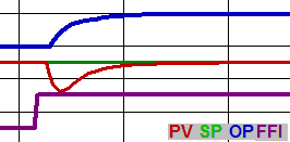
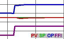
For most loops, the transition between modes – between auto, manual or tracking, and between remote (cascade) or local – should be made without causing a bump (a step-change) to the OP. A ramping SP makes this easy – when in manual (or output tracking), the ramping SP should track the PV so that when the loop is returned to auto, it will ramp from where it is to the target SP.
For cascaded loops – or any loop with additional logic downstream, rather than the OP simply driving an AO – output tracking is essential. If the slave loop is in any mode other than auto-remote (cascade), the master OP must track the slave’s SP (which tracks the slave’s PV if in manual or OP-tracking) so that it doesn’t bump the slave’s SP when it returns to auto-remote.
In some cases, there are additional functions between a master and slave which makes the master OP tracking the slave’s SP complicated. For example, there may be a piecewise curve between the master and slave. In that case, rather than attempting to run the functions backward, it may be more simple to implement an integral-only loop to continuously adjust the tracking OP so that the result of the functions is close to the slave loop’s SP. This may result in a very small bump when returning to auto-remote, but it would probably not be noticeable.
Single and Three Element Control
The classic example of a three-element (3E) control system is boiler drum level. Three key process variables are measured:
- The drum level.
- The feedwater mass-flow to the drum.
- And the mass-flow of steam out of the drum.
As discussed above, the drum level is the PV for the master PID loop, the feedwater flow is the PV for the slave PID loop (which drives the feedwater valve), and the steam flow is the FF input to the master loop. In such a system, at low flow rates the three element control system does not work well, so the system switches to “single element” (1E) where the OP of the level loop runs directly to the feedwater valve.
The system should be able to automatically make bumpless switches between 1E and 3E control. To accomplish this it is best to have two separate level PID blocks: one for 1E and one for the 3E master. The 3E slave flow OP is always set from the 3E level master OP regardless of mode. When in 1E, the following values should track:
- The 3E level master SP tracks the 1E loop’s SP.
- The 3E level master OP tracks the measured feedwater flow rate.
- The 3E flow slave OP tracks the 1E loop’s OP.
When in 3E, the following values should track:
- The 1E loop’s SP tracks the level master’s SP.
- The 1E loop’s OP tracks the 3E flow slave loop’s OP.
In this way, the OP going to the valve is always the same for both loops. Force the 3E slave to always be in remote-auto (cascade), and drop the system to 1E if the 3E master level loop is placed in manual.
The operator should have a “3E enable” switch allowing him to force the system to 1E, or enable the system to automatically switch between modes. When enabled, the system should switch after a delay after both flows are good quality and above a “1E maximum flow”. It should drop back to single element immediately if either flow quality goes bad, or either drops below a “3E minimum flow” set somewhat below the 1E maximum flow, to give the switching logic some deadband.
Having two PID blocks for the same PV represents a challenge when opening an HMI popup faceplate – usually I hide the touch-point for the inactive loop so that if the loop is clicked when in 1E, the faceplate for the 1E loop appears, but if in 3E control, the faceplate for that master appears instead.
For more details on this control scheme, please read Three Element Drum Level Control.
Smoothing Filters
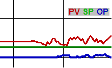
Many loops have noisy PV or FF inputs. Noise translates directly to the OP through the proportional, derivative, and feed forward algorithms. I prefer smoothing the inputs over ramping the outputs. But rather than smoothing the raw PV, I prefer to leave it noisy so operators can see what it is actually doing, and smooth the signals internally before sending them to the PID block. If a controller does not have a smoothing filter function, a simple exponential-decay filter is easy to construct: each scan, add 0.99 times the previous signal to 0.01 times the new signal. Change the 0.99 closer to 1 to make the signal smoother (the 0.01 must be changed to 1 – the replacement for 0.99).
There is a trade-off between a responsive loop and a smooth OP – too much smoothing will cause the loop to be sluggish.
Non-Linearity, Characterization, and Adaptive Gain Control
For many loops, the OP is not linear to PV. For example, moving a damper from 5% to 10% might result in an increase of air flow from 100 k#/H to 150 k#/H, while a move from 80% to 85% might only change it from 400 k#/H to 405 k#/H. This presents a problem to a standard PID loop – either the loop is well tuned at low flows but very sluggish at high flows, or it is well tuned at high flows but wildly unstable at low flows.
Characterizing the output device
One traditional way of compensating for this non-linearity to achieve responsiveness and stability through the entire flow range is to characterize the output device by implementing in the logic a piecewise curve between the PID’s OP and the analog output (AO) to the device. In the above example, a 20% OP might be converted to a 5% AO, 30% OP to 10% AO, 97% OP to 85% AO, and 98% to 90% AO. This approach works well, but can be confusing to the operator because when a 30% OP is entered into a loop in manual, the damper would move to its 10% mark. This also has the disadvantage of the characterization curve having to be adjusted as the device wears to retain good control.
Adaptive Gain Control has advantages over Characterization
Adaptive gain control allows you to solve the same problem without resorting to a curve. Many modern PID blocks have a “gain modifier,” which when set to 1, runs the loop as normal, but when set to 2, doubles each of the three actions relative to their nominal constants. In this example, the programmer might configure the gain modifier to (1 + OP * 10). The nominal tuning constants would be used when the damper is closed, and as the damper opens, the loop becomes more and more responsive. This has the advantages of:
- Using the actual output to the damper so that there is no confusion over which % the operator is manipulating.
- The loop still performs well even if the damper characteristics change due to wear or other changing conditions.
- Time saved by not having to enter the characterization into the controller.
Use Adaptive Gain to compensate for other changes to responsiveness
Adaptive gain control is also useful for situations where a loop’s responsiveness needs to change because of variable pumps or fans. For example, if just one pump in a pair is running to a valve on the common header, that valve needs to be more responsive than when both pumps are running. The gain modifier could be set to 1 when one pump is running, and automatically changed to 0.7 or 0.6 when both are running.
Use Adaptive Gain to schedule tuning for different control zones
You can use adaptive gain (or different sets of the tuning constants) to separately tune a loop for different situations. For example, in batch control, it may be beneficial to have different tuning for when a temperature is ramping (heating up) than when it is soaking (holding steady at the target temperature). Delaying or ramping the switchover to steady state tuning constants may be necessary to compensate for the time the heat takes to saturate the unit at the new temperature.
Another approach to ramp/soak control (especially if the ramp time is unimportant and you just want to get to the target temperature as fast as possible, given various limits) is to force the loop’s OP to track an externally calculated value based on the distance from the target SP heating, then release to auto around when it reaches the target, with the loop optimally tuned only for steady-state control.
Integral Windup, Ramping and Clamping
Standard PID loops may suffer from integral windup when an OP is clamped and/or after a large SP change. On a large SP change, the proportional makes a corresponding change, and then while the PV is still far from the SP the integral action accumulates. This “double action” can cause the PV to overshoot while the integral “unwinds”. One very simple, practical way to prevent that kind of windup is to always ramp SP changes. Have the operator enter a target SP, and have the SP of the loop ramp to that target instead of jumping to it.
Ramp with Terminal Deceleration
Standard ramps run linearly until reaching the target & then stop.
This can cause a small overshoot that is easily avoided by a terminal deceleration – rounding off the end of the ramp. Multiply the difference between the ramping and target SPs by a constant. (This alone would result in a purely asymptotic ramp). Then, if that ramp amount exceeds the maximum ramp rate, clamp it to that maximum.
Setpoint Outrun Prevention
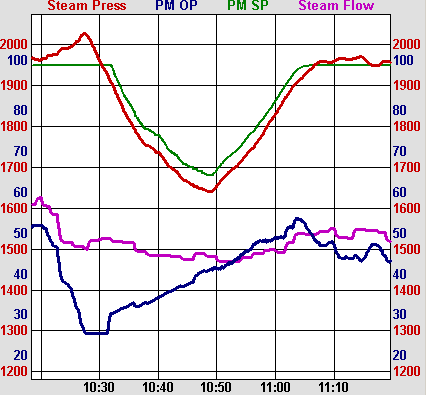
Use SP ramp outrun prevention for ramping SPs to avoid overshooting and/or the OP rising to its upper clamp. To implement this feature, if the ramping SP is more than a certain amount above the PV, set it that amount above the PV. For example, a boiler steam pressure controller’s OP drives the rate of fuel. It would cause problems in the furnace for the fuel OP to rise all the way to its high clamp from a low value. Outrun prevention allows rapid responses of moderate amounts in fuel OP to steam pressure changes within the outrun band – but after that, this feature intentionally allows the PV (steam pressure) to slump rather than put too much fuel into the furnace and risk an overshoot or other problems. Typically outrun prevention is one-sided – in this case the ramping SP might not be allowed to rise more than 40 PSI above the PV, but could be any amount below the PV.
Clamped Outputs
Another aspect of windup is what happens when an OP is clamped at its limit. Some controllers just clamp the OP and apply the actions on the next scan to that clamped OP. Other controllers maintain an internal OP which can go beyond the clamp. Typically only the proportional will be applied to that internal when it is beyond the limits – no integral would be applied.
Both of these approaches have drawbacks. The clamp-only approach will not stay settled at the limit if there is any noise on the PV because the proportional will “ratchet” the OP away from the limit as it bounces back and forth. The unclamped internal OP can result in the OP staying at its limit far longer than it should when the PV starts heading back toward the SP, resulting in a significant overshoot.
One way to avoid both problems is to clamp the external OP, then also clamp the internal a few % outside the external clamp. So an OP clamped 0% to 100% might have an internal clamp of -2% to 104%. This allows the OP ratcheting which occurs from typical PV noise to occur between the clamps so that the external OP stays right at its clamp, but is ready to respond quickly once the PV starts returning to the controllable range. Some PID blocks support this feature. For the majority of blocks that don’t, an easy way to achieve it is to set the PID block’s OP clamps to the outer settings (such as -2% to 104%), then send that OP through a clamp external to the PID block before it reaches the analog output or other logic.
Avoid Trips with Raise and Lower Inhibits
Some loops might have an OP clamp set 0% to 100%, but under some conditions can cause problems within that range. For example, the steam pressure controller for a boiler can call for more fuel to the furnace than other parts of the boiler can handle. A fan might be at the limit of how much air it can deliver, or a feedwater valve fully open, or a temperature too high, or some other device might be at an operating limit.
Rather than trip the system, raise and lower inhibits can be used to allow the system to approach but not exceed any of its limitations. Each potential limiting factor should have a flag indicating when it is about to be reached, and the OP of the main loop driving the whole system (in this case main steam pressure) inhibited from rising when any of the flags are set. These flags might take the form of an air flow being more than 2% below SP, a valve being more than 95% open, a temperature within 5° of its high warning limit, etc.
Some loops have an input for raise and lower inhibit. For those that don’t, this can be implemented by setting the OP high limit to a constant (such as 100%) when not raise inhibited, and set to the current OP when any raise inhibit condition is in effect.
The result of a raise inhibit may not be noticeable if the condition is intermittent. Using the dual OP clamps discussed in the windup section would allow the OP to jump up a bit when the inhibit is released, retaining good control. However, when a system demand really exceeds what it can deliver, the result will be that the PV of the loop will slump below its SP – but that is preferable to allowing it to try to maintain its SP at the cost of a trip. In the example of a boiler, if the inhibit stays in too much, the steam pressure will drop below SP. The operator must then either reduce steam demand (perhaps by throttling back a turbine generator) or resolve the limiting factor (perhaps by starting another pump or fan).
Runbacks
In a few cases, merely inhibiting an output may not be sufficient to prevent a system from tripping. It may be necessary to run back the OP in a condition approaching the trip point. Runback logic can be treated similarly to a raise inhibit, except the output limit ramps down instead of holding. Alternatively, if the runback is due to a tripped piece of equipment (perhaps if one of a pair of pumps trips), the output may need to be suddenly stepped down to a much lower limit. This would obviously upset the system but could be preferable to a trip.
Chopping Outputs on a Duty Cycle
Sometimes an OP does not do well below some positive value. For example, a valve may suddenly raise the flow from zero to ¼ of full range flow when moving from 3% to 4%. A VFD may not be able to run below 15 Hz without overheating the motor. In these cases, the analog OP of a PID loop can be run through a chopping / duty cycle function: Have a duty cycle timer that resets periodically.
If the OP is above the minimum, ignore the timer and just send the OP to the AO device. If the OP is below the minimum, set it to the minimum for the proportion of the duty cycle corresponding to OP / OP_Min, then set it to zero (and stop VFDs if applicable) for the remainder of the duty cycle.
Fixed Proportional
Many tank levels are acceptable anywhere in a fairly wide range. If tuning the level to achieve a stable OP is difficult, an alternate algorithm may help – this is essentially just the proportional term from the PID with fixed range. Set up a minimum and maximum level PV, and a minimum and maximum OP. When the PV is outside the min-max range, clamp the OP to its min or max. In between, scale off linearly using a standard scale block or with the mapping function:
OP = (PV – PV_Min) * (OP_Max – OP_Min) / (PV_Max – PV_Min).
For systems requiring the OP to fall when PV rises, use:
(PV_Max – PV) instead of (PV – PV_Min).
Hold-Jump Loops
Another alternate feedback algorithm to PID is the “hold-jump” loop. This is useful for controlling flow when there is an acceptable range around an SP, and the flow valve has a lot of hysteresis (a much different PV is seen when moving the OP down to a value versus up to the same value) and/or control deadband, where a motorized valve waits for a large OP change before moving.
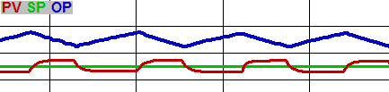
Smoothing the PV is important for a hold-jump loop – you don’t want it to jump due to a blip on the PV. Set a deadband (DB) where if the PV is within SP±DB, no change will be made. When the PV goes outside SP±DB, calculate the new OP by multiplying the loop’s gain by the error. Then drop the OP by a prescribed amount (perhaps 5%) below the new OP and hold it there for a second or so, then take it up to the new OP. This defeats both hysteresis (by always approaching the new value from the same direction) and deadband (by always making large changes).
After a change, hold the OP for some time (perhaps 15-30 seconds) even though the PV is outside the SP±DB for part of that time.
An advanced option is to start the DB after a jump at a larger value and have it ramp or decay to a smaller final value. That allows the loop to be more responsive to very large error more quickly, yet keep the PV closer to the SP with fine changes in the long run.
While this is useful for primary feed flows intended to be roughly constant, it would not do well for flows with SPs that frequently move around. Hold-Jump loops tend to not be responsive to upsets.
Better Loop Tuning with Advanced Methods
- Use cascaded loops to achieve better control of slow master PVs when a faster (usually flow) PV can be controlled by the device. The fast slave loop linearizes the master loop’s OP and eliminates hysteresis.
- Use feed forward to adjust the OP of a loop to minimize an upset after a measurable external value changes.
- Use trim control instead of cascade with feed forward if the deviation from demand should be limited and the exact master PV has a band of acceptable values.
- Use bumpless transfer to prevent transitions between modes from causing process upsets.
- Smooth PV and FF inputs to reduce OP noise.
- Use adaptive gain to compensate for non-linear OP devices and other conditions that affect loop responsiveness.
- Ramp Setpoints, use SP outrun prevention and allow internal OPs to slightly exceed external OP clamps to avoid overshooting due to integral windup.
- Use raise and/or lower inhibits and runbacks to allow PVs to slump away from SPs when that is preferable to a major system trip.
- Use unconventional algorithms when physical limitations prevent a standard PID loop from working well.
- Combine these advanced methods with good basic tuning to achieve a stable, responsive, minimally overshooting loop.
Work With an Expert
If you are experiencing issues with tuning your PID loop we encourage you to reach out to one of our process solutions experts. While this guide is intended to help you tune your PID loop and troubleshoot common issues, this is not an exhaustive list. Please contact us today to discuss your application and specific issues you may be having with your PID loop.