Square Root Scaling for Differential Pressure (DP) Flow Meters
Instruments should be ranged to measure not only expected values but all values the system can produce. During upsets, actual values often exceed 20mA values for instruments tightly ranged for normal process conditions. For instruments with linear scale and additional capacity, the fix is simple: increase the 20mA scale on both the instrument and analog input (AI) in the controller. But nonlinear relationships complicate scale adjustments.
Nonlinear Flow Measurement
Most methods of flow measurement are nonlinear. Some calculations are always handled inside the transmitter (mag-meters, Coriolis, Vortex, etc) so that the mA signal is linear to flow for those types of meters. But the most common method of flow measurement is differential pressure (DP) across an obstruction. Regardless of the type of obstruction (orifice plate, Venturi or Pitot tube, etc), the DP is proportional to the square of the flow. Therefore the system must scale flow from the square root of the DP.
The square root for DP-based flow can be taken either in the transmitter or in the controller (but not both!). We prefer to configure the transmitter to take the square root because, on the low end, a very small change in DP results in a large change in flow. This makes low flows extra sensitive to electrical noise on the mA signal if the square root is taken in the controller.
Logic for Taking the Square Root in the Controller
If it is not feasible to take the square root in the transmitter, and you are writing your own square root scaling logic in a controller instead of checking a square root option in a standard function block, then follow these steps.
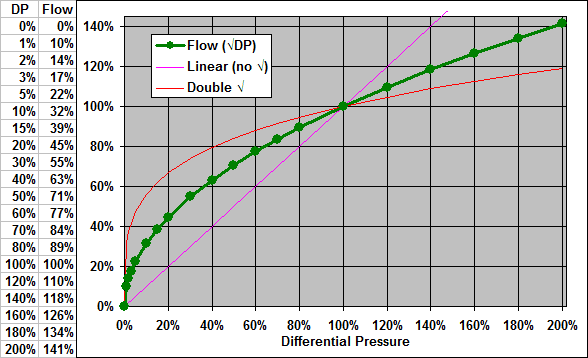
First, normalize the signal to 0-1, where 0 is 4 mA, 1 is 20 mA, and 0.5 is 12 mA. The square root then makes sense, as the root of a number >1 is smaller than the number. But the root of a number from 0-1 is larger: √0.5 = 0.707. So if you have a 12 mA signal from the DP cell, that’s 50% DP, but 71% flow rate. Multiply the resulting square rooted signal (still 0-1) by the flow scale span to get flow rate in engineering units.
The square root of a negative number is imaginary, and will cause most processors to throw a minor fault and declare the result “Not A Number.” To avoid these problems, either clamp negative normalized inputs to zero or square root the absolute value and make it negative again if the original was negative (below 4mA).
Scaling Flow to DP From a Flow Data Sheet
Typically, a flow element such an orifice plate or Venturi tube will come with a flow data sheet with expected process conditions and a table of flow rates for various DPs. The only number important for scaling is the highest flow/DP pair on the sheet. For basic scaling, set the range of the DP transmitter from zero at 4mA to the highest DP on the sheet at 20mA. Then in the controller, scale the input from zero at 4mA to that maximum flow at 20mA. If the square root is taken in either the transmitter or controller (but not both), the system will correctly calculate flow through the range of the meter.
Checking Scaling and Square Root Configuration
Checking the zero and full span DP, calibrating 4mA and 20mA, and verifying that the controller displays the correct flow at 4mA and 20mA is necessary but insufficient to verify square root configuration. You must also apply one or more of the mid-range DPs from the flow data sheet to the meter and verify that the controller displays the correct flow rate.
Generally, if any mid-range value is correct (along with the zero and maximum), they will all be correct, following the green curve in our chart. If a mid-range flow displays significantly lower than it should have (see the magenta line in the chart), the square root may not be implemented anywhere. If it is significantly higher (see the red curve in the chart), you may be taking the square root on both ends.
See How Our Team Can Help Improve Quality, Increase Efficiency, And Reduce Risk In Your Operation
Correcting for Process Conditions Which Affect Density
A DP meter measures fluid velocity, yielding volumetric flow (GPM, CFM, etc) when multiplied by the cross sectional area of the duct or pipe. Fluid density is irrelevant to that measurement and calculation. Mass flow (#/H, SCFM, etc) is calculated by multiplying volumetric flow by density. For the most accurate mass flow, if any of the nominal process conditions on the flow data sheet differs from actual conditions in a way that significantly affects density, the flow should be compensated.
- Ideal gases (such as air, natural gas, etc) increase in density linearly with rising pressure and falling temperature.
- Non-ideal gases (steam) also increase in density with rising pressure and falling temperature, but not linearly, so density values must be determined from tables or curves approximating tables.
- Liquid density is not significantly affected by changes in pressure but, usually, drops with rising temperature. There are exceptions (water from 32°F to 39°F). There is only a 2% difference in density between water at 39°F and water at 150°F, so differences in that range are probably not worth compensation. However, water at 212°F is 4% less dense than at room temperature, and water at 400°F is 14% less. Therefore, at higher temperatures, a deviation between nominal and actual temperature may be significant enough to compensate. Liquid density versus temperature is almost always nonlinear – look it up from a table or curves approximating a table.
To compensate mass flow for density, we recommend the following logic:
- Use a density function block with inputs for all significant parameters (pressure and temperature for gases, or just temperature for liquids). The inside of that block will depend on the type of fluid.
- Attach nominal conditions from the flow data sheet as constants to an instance of the density block. The result will be “nominal density.”
- Attach actual conditions to another instance of the density block. The result will be “actual density.” Conditions ideally are measured with pressure and temperature instruments, but either or both can be entered as constants if that information is not available to the controller.
- Compensated mass flow = [Raw uncorrected mass flow] x [actual density] ÷ [nominal density]
Increasing The Scale
If the actual flow exceeds the maximum scale – even during an upset – you should increase the scale so that these values can also be measured. For a square rooted flow, some math is involved, as DP increases with the square of the flow.
This re-scaling will result in some loss of measurement precision, but, typically, that loss is still far lower than measurement noise and so is not relevant. The hard limit on increasing scale is the limit of the transmitter. Many DP cells for flow measurement are nominally scaled 0-100″WC (inches water column), and the transmitter may be able to measure up to 200″ or 300″, but no higher.
The simplest way to re-scale is to determine how much more flow you need, represent that as a multiplier, then square it for the change in DP.
Example
- If 100″WC is 1000 GPM, and you need to measure 1190 GPM, you need 20% more scale, so your multiplier is 1.2.
- 1.2 x 1000 GPM is 1200 GPM.
- 1.2² = 1.44, x 100″WC is 144 “WC.
- You can increase your transmitter range from 100″WC to 144″WC, your controller AI scale from 1000 GPM to 1200 GPM, and the system will still read flow properly.
You can also increase DP by a multiple, then increase the flow scale by the square root of that multiple. This is how to calculate the highest possible flow measurement for a given transmitter limit.
Example
- If your transmitter can measure up to 225″WC, while nominal maximum DP is 100″WC, the DP multiplier is 2.25.
- √2.25 = 1.5, x 1000 GPM = 1500 GPM.
- That is the highest flow your DP cell can measure
Pulse Meter Scaling
Some flow meters (particularly turbine meters and any revenue meter) output flow as a discrete pulse for every given unit of volume or mass. The flow data sheet for such a meter will typically list the volume per pulse or may invert to give pulses per a unit volume.
Example
- A flow data sheet lists 228 pulses per gallon.
- This is the same as 0.004386 (1 ÷ 228) gallons per pulse
If you are configuring a standard function block or pulse-to-4-20mA transmitter, you need to determine your maximum scaled flow rate. Note that this is NOT your expected flow rate – it must be well higher than expected to properly deal with upset conditions. In this example, 20 GPM was the maximum nominal flow, so we want to scale the transmitter to 30 GPM. 228 Pulses/Gal x 30 GPM = 6840 Pulses/Min ÷ 60 Sec/Min = 114 Pulses/Sec or Hz. So 114 Hz is equivalent to 30 GPM.
If you are bringing the pulse signal directly to a discrete input (DI) on the controller, calculating the total is trivial – just add the volume per pulse to an accumulator every time you see a new pulse (with one-shot/rising edge detection). Calculating flow rate is more complicated – there are two general ways to do that:
For slower pulses that last many (at least 10) processor scans, measure the time between pulses. Continuously run a timer. On a new pulse (rising edge), divide the time base by the accumulated time, then reset the timer.
- So in this example, if your timer is running in milliseconds, and you want gallons per minute, your time base is 60000 (milliseconds per minute).
- Divide 60000 ÷ time elapsed since the last pulse.
- Multiply that by the volume per pulse. So if you had a pulse lasting two seconds, or 2000 ms, that would be 0.004386 x 60000 ÷ 2000, or 0.13 GPM.
- You must also set a maximum time limit – this is a standard feature on a timer – the “preset.” If the timer reaches the preset and is “DONE”, set the resulting flow rate to zero. Without this step, the flow would indefinitely continue to be reported as the last positive flow before it stopped flowing and pulsing.
For faster pulses, count the pulses in a fixed time period, and multiply that by a time multiplier and the volume per pulse multiplier. If the pulses are coming more often than once every two scans, this will require a high-speed counter DI (which counts pulses and reports the count per scan to the processor) since the processor would miss pulses just looking at the raw DI. In this example, you might program the processor to count pulses every second. You’d multiply that by 60 to convert seconds to minutes, and by also 0.004386 to get GPM.
Totalization
Totalized flow is an important value for most flow meters. If your flow meter is attached via HART or some other communication protocol, you may be able to read the flow total from the meter. Otherwise, you will need to calculate it in the controller using an accumulator. If you calculate a total for one hour, a work shift, or a day, then roll that into a previous register, a standard totalizer will work.
However, a grand total with an accumulator stored in a 32-bit floating point (a “float”) will stop working after a while due to rounding error. A float has a precision of about 1 part in 16,000,000. If you add 1 to 16,000,000 into a float, the result will be 16,000,001 as expected. But if you add 1 to 17,000,000, it’s going to round back down to 17,000,000. So, a totalizer will quit accumulating altogether after 16,000,000 scans and will have been inaccurate for a while before that. 16,000,000 seconds is about 6 months, but many controllers scan many times per second, significantly reducing the time until such a totalizer would quit.
To solve this problem, use three registers for a grand totalizer: Accumulate a “current hour total.” At the end of the hour, add that result to the “all previous hours” register, then reset the current hour total register. The grand total will always be those two registers added together.
If your controller has a 64-bit floating point register, use that – they have a precision of 1 part in about 9,000,000,000,000,000, so they don’t suffer from the same problem.
Summary
- Many methods of flow measurement have a nonlinear relationship between the measured value and the rate of flow.
- While re-scaling a linear signal is trivial, re-scaling a nonlinear signal requires an appropriate adjustment.
- Flow scales should be checked against the flow data sheet at a minimum of three points (zero, maximum, and a point in between) to verify the proper configuration.
- If actual conditions differ from the nominal ones on the flow sheet, density compensation may be appropriate.
- Flow meters with pulse outputs are easy to totalize. There are also methods to calculate flow rate from the timing of a pulse input.
- Simple totalizers for a limited time work fine, but a grand total stored in a 32-bit floating point value will eventually stop working due to rounding error – multiple registers may, therefore, be needed.
For more information about Square Root Scaling for Differential Pressure (DP) Flow Meters, contact our team and discuss your application.